Linux-Memory-Management

阅读更多

1 Virtual Memory

摘录自20 张图揭开「内存管理」的迷雾，瞬间豁然开朗

The CPU of a microcontroller directly operates on memory using ‘physical addresses’

In this scenario, it is impossible to run two programs simultaneously in memory. If the first program writes a new value at position 2000, it will overwrite all the content stored in the same location for the second program. Therefore, running two programs simultaneously is fundamentally impossible, and both programs will crash immediately.

How does the operating system solve this problem?

The key issue here is that both of these programs are referencing absolute physical addresses, which is exactly what we need to avoid.

We can isolate the addresses used by processes, meaning that the operating system allocates a separate set of virtual addresses for each process. Everyone gets their own set of addresses to play with, and they don’t interfere with each other. However, there’s one condition: no process can directly access physical addresses. As for how virtual addresses ultimately map to physical memory, it’s transparent to the processes; the operating system takes care of all these arrangements.

The operating system provides a mechanism to map the virtual addresses of different processes to different physical memory addresses.

When a program accesses a virtual address, the operating system translates it into a distinct physical address. This way, when different processes run, they write to different physical addresses, avoiding conflicts.

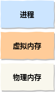
So, this introduces two concepts of addresses:

• The memory addresses our programs use are called Virtual Memory Addresses.
• The spatial addresses that actually exist in hardware are called Physical Memory Addresses.

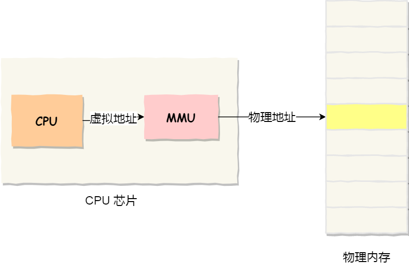
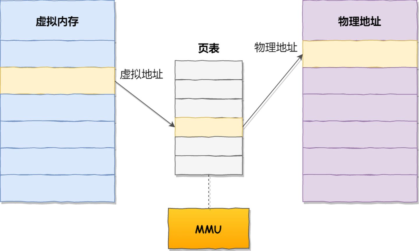
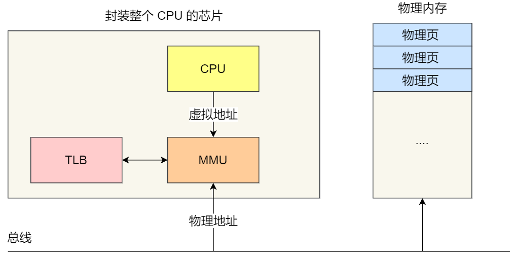
The operating system introduces virtual memory, where the virtual addresses held by a process are translated into physical addresses through the mapping relationship of the Memory Management Unit (MMU) within the CPU chip, and then memory is accessed via the physical address, as shown in the diagram below:

How does the operating system manage the relationship between virtual addresses and physical addresses?

There are primarily two methods: memory segmentation and memory paging. Segmentation was proposed earlier, so let’s first take a look at memory segmentation.

2 Memory Segmentation

摘录自20 张图揭开「内存管理」的迷雾，瞬间豁然开朗

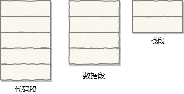
A program is composed of several logical segments, such as code segments, data segments, stack segments, and heap segments. Different segments have different attributes, so they are separated using segmentation.

In the segmentation mechanism, how are virtual addresses mapped to physical addresses?

In the segmentation mechanism, a virtual address consists of two parts: the segment selector and the offset within the segment.

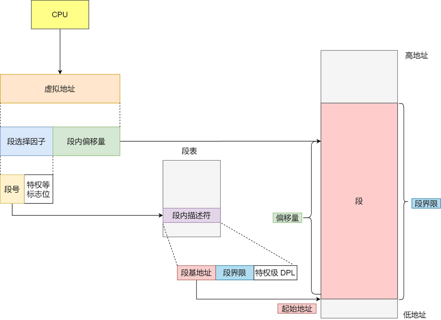
• The segment selector is stored in a segment register. The most important part of the segment selector is the segment number, which is used as an index into the segment table. The segment table contains the base address of the segment, segment limit, and privilege level, among other information for that segment.
• The segment offset in the virtual address should be between 0 and the segment limit. If the segment offset is valid, it’s added to the segment’s base address to obtain the physical memory address.

In the above explanation, we learned that virtual addresses are mapped to physical addresses through the segment table. The segmentation mechanism divides the program’s virtual address into four segments, with each segment having an entry in the segment table. In this entry, you can find the base address of the segment. By adding the offset to this base address, you can locate the address in physical memory, as illustrated in the following diagram:

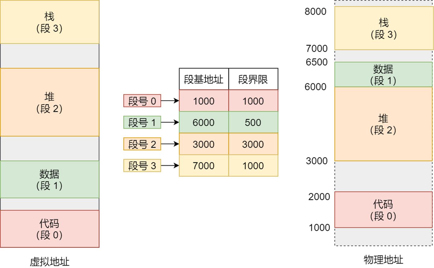
If you want to access the virtual address with offset 500 in segment 3, you can calculate the physical address as follows: Segment 3 base address 700 + offset 500 = 7500.

Segmentation is a good approach as it resolves the issue of programs not needing to be concerned with specific physical memory addresses. However, it has a couple of shortcomings:

1. The first issue is memory fragmentation.
2. The second issue is inefficient memory swapping.

Let’s discuss why these two problems occur.

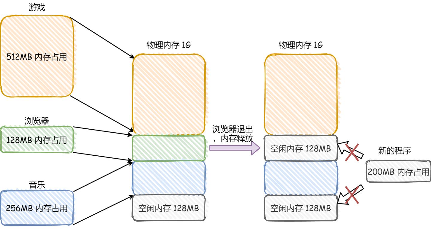
Consider this example: Suppose there is 1GB of physical memory, and users are running multiple programs:

• A game occupies 512MB of memory.
• A browser occupies 128MB of memory.
• Music occupies 256MB of memory.

Now, if we close the browser, there will be 1024 - 512 - 256 = 256MB of free memory. If this 256MB is not contiguous and is split into two segments of 128MB each, it would lead to a situation where there is no space available to open a 200MB program.

The issue of memory fragmentation in this context occurs in two ways:

1. External memory fragmentation, which results in multiple non-contiguous small blocks of physical memory, preventing the loading of new programs.
2. Internal memory fragmentation, where all of a program’s memory is loaded into physical memory, but some portions of that memory may not be frequently used, leading to memory waste.

The solutions for addressing these two types of memory fragmentation are different.

To tackle external memory fragmentation, we use memory swapping.

In memory swapping, the 256MB of memory occupied by the music program is written to the hard disk and then read back into memory from the hard disk. However, when reading it back, it cannot be loaded back into its original location; instead, it is placed immediately after the already occupied 512MB of memory. This frees up a contiguous 256MB space, allowing a new 200MB program to be loaded.

This memory swapping space, often referred to as Swap space, is allocated from the hard disk in Linux systems and is used for the exchange of data between memory and the hard disk.

Now, let’s take a look at why memory swapping is less efficient with segmentation.

For multi-process systems, using segmentation can easily lead to memory fragmentation. When fragmentation occurs, we have to perform memory swapping (Swap), which can create performance bottlenecks.

This is because accessing the hard disk is much slower compared to memory. During each memory swap, we need to write a large contiguous block of memory data to the hard disk.

So, if the memory swap involves a program that occupies a large portion of memory, the entire system can become sluggish.

To address the issues of memory fragmentation and low memory swapping efficiency with segmentation, memory paging was introduced.

3 Memory Paging

摘录自20 张图揭开「内存管理」的迷雾，瞬间豁然开朗

Segmentation has the advantage of creating contiguous memory spaces but can lead to memory fragmentation and inefficient memory swapping due to large spaces.

To address these issues, we need to find ways to minimize memory fragmentation and reduce the amount of data that needs to be swapped during memory exchange. This solution is known as Memory Paging.

Paging involves dividing the entire virtual and physical memory spaces into fixed-size chunks. Each contiguous and fixed-size memory space is called a page. In Linux, the size of each page is typically 4KB.

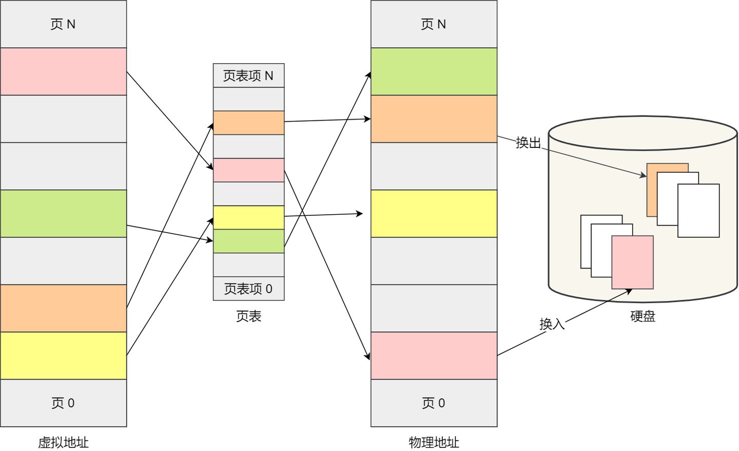
Virtual addresses are mapped to physical addresses using a page table, as shown in the diagram below:

The page table is actually stored in the Memory Management Unit (MMU) of the CPU. Therefore, the CPU can directly access the physical memory address to be accessed through the MMU.

When a process accesses a virtual address that cannot be found in the page table, the system generates a page fault exception. It enters the kernel space of the system, allocates physical memory, updates the process’s page table, and then returns to the user space to resume the process’s execution.

How does paging solve the issues of memory fragmentation and low memory swapping efficiency seen in segmentation?

With paging, memory spaces are pre-allocated, and there are no small gaps as seen in segmentation, which is the reason for memory fragmentation in segmentation. In paging, released memory is released in page-sized units, avoiding the issue of small unusable memory blocks.

If there isn’t enough memory space, the operating system will release pages of memory from other running processes that have not been recently used. This is known as swapping out. When needed again, these pages are loaded back into memory, known as swapping in. Therefore, only a few pages or even just one page are written to disk at a time, which doesn’t take much time. As a result, memory swapping is more efficient.

Furthermore, the paging approach allows us to load programs into physical memory gradually, rather than all at once when we load a program. We can map virtual memory pages to physical memory pages and do not need to load pages into physical memory until they are actually needed during program execution.

How are virtual addresses and physical addresses mapped under the paging mechanism?

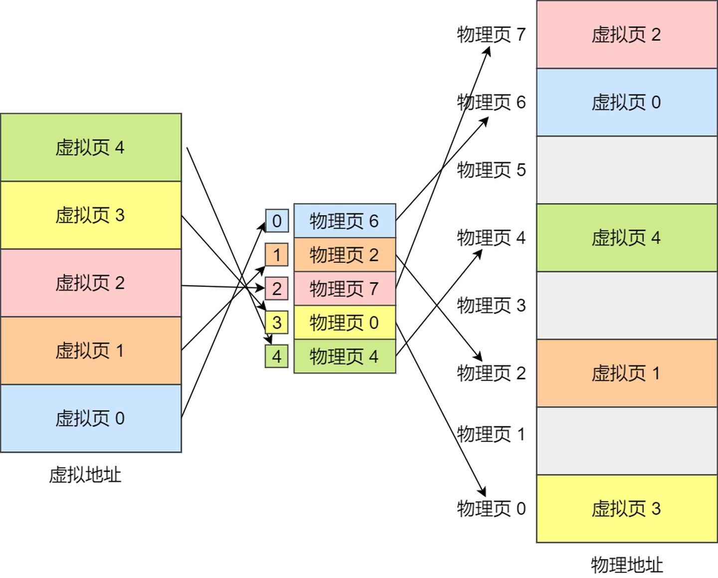
In the paging mechanism, a virtual address is divided into two parts: the page number and the page offset. The page number serves as an index for the page table, and the page table contains the base addresses of each physical page in physical memory. The combination of this base address and the page offset forms the physical memory address, as illustrated in the diagram below:

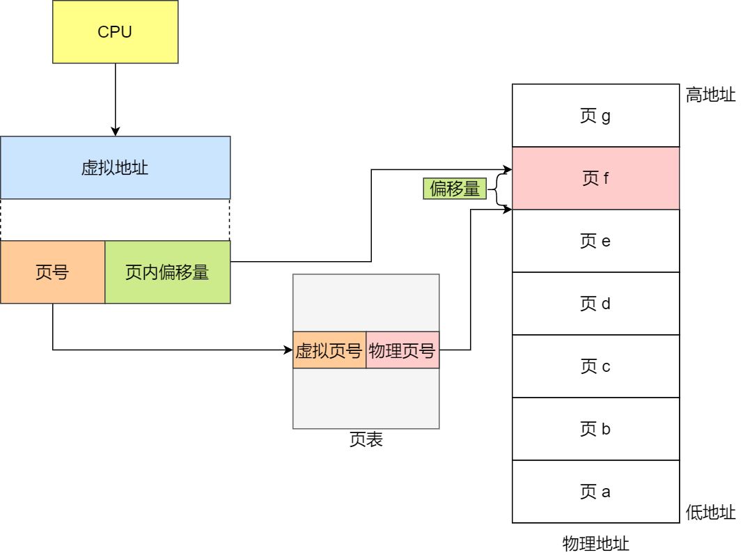
To summarize, the process of memory address translation involves three steps:

1. Splitting the virtual memory address into a page number and an offset.
2. Using the page number to look up the corresponding physical page number in the page table.
3. Directly adding the physical page number to the offset to obtain the physical memory address.

Here’s an example: Virtual memory pages are mapped to physical memory pages through the page table, as illustrated in the diagram below:

This may seem fine at first glance, but when applied to real-world operating systems, this simple paging approach does have limitations.

Are there any shortcomings to simple paging?

One significant limitation is space-related.

Since operating systems can run many processes simultaneously, this implies that the page table will become very large.

In a 32-bit environment, the virtual address space is 4GB. If we assume a page size of 4KB (2^12), we would need around 1 million (2^20) pages. Each “page table entry” requires 4 bytes to store, so the entire mapping of the 4GB space would require 4MB of memory to store the page table.

This 4MB page table size may not seem very large on its own. However, it’s essential to note that each process has its own virtual address space, meaning each has its own page table.

So, for 100 processes, you would need 400MB of memory just to store the page tables, which is a substantial amount of memory. This issue becomes even more significant in a 64-bit environment.

To address the problem mentioned above, a solution called “Multi-Level Page Table” is needed.

As we discussed earlier, with a single-level page table implementation, in a 32-bit environment with a page size of 4KB, a process’s page table needs to accommodate over a million “page table entries,” each taking up 4 bytes. This implies that each page table requires 4MB of space.

To overcome this limitation, we can introduce a multi-level page table, where the first-level page table is divided into 1024 second-level page tables, with each second-level table containing 1024 “page table entries.” This creates a two-level paging system, as illustrated in the diagram below:

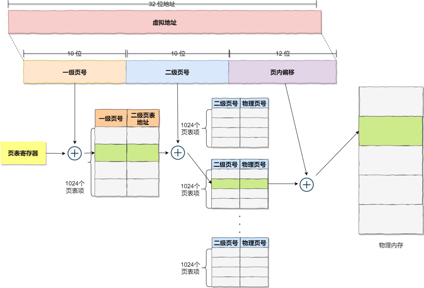
You might be wondering, by introducing a two-level page table, aren’t we consuming more memory? Mapping the entire 4GB address space would indeed require 4KB (first-level page table) + 4MB (second-level page table), which seems larger.

However, we should look at this from a different perspective, and remember the ubiquitous principle of locality of reference in computer architecture.

Each process has a 4GB virtual address space, but for most programs, they don’t utilize the entire 4GB. Many page table entries may remain empty, unallocated. Furthermore, for allocated page table entries, if there are pages that haven’t been accessed recently, the operating system can swap them out to the hard disk, freeing up physical memory. In other words, these pages do not occupy physical memory.

With two-level paging, the first-level page table can cover the entire 4GB virtual address space, but if a page table entry is not used, there’s no need to create the corresponding second-level page table until it’s needed. Let’s do a simple calculation. Suppose only 20% of the first-level page table entries are used. In that case, the memory occupied by the page tables would be 4KB (first-level page table) + 20% * 4MB (second-level page table) = 0.804MB. This is a significant memory saving compared to the 4MB used by a single-level page table.

So, why can’t single-level page tables achieve this memory saving? Looking at the nature of page tables, they are responsible for translating virtual addresses into physical addresses and are vital for the computer system to function. If a virtual address cannot be found in the page table, the computer system cannot operate. Therefore, page tables must cover the entire virtual address space. Single-level page tables would require over a million page table entries to map the entire virtual address space, while two-level paging only needs 1024 page table entries (with the first-level page table covering the entire virtual address space and second-level page tables created as needed).

When we extend this concept to multi-level page tables, we realize that even less memory is occupied by page tables. All of this can be attributed to the effective utilization of the principle of locality of reference.

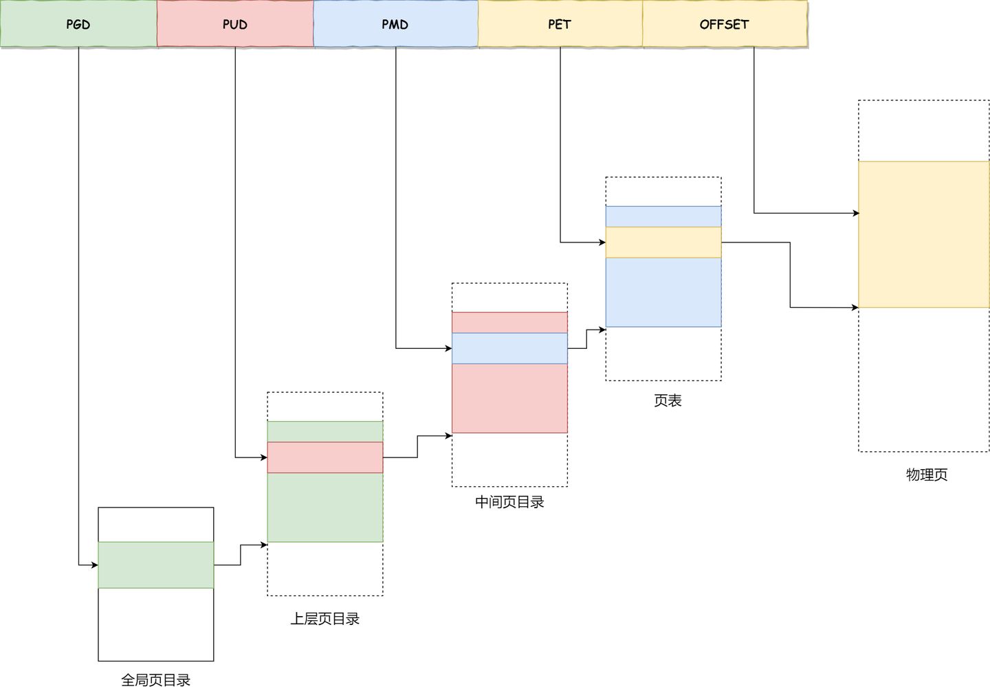
In a 64-bit system, two-level paging is insufficient, so it becomes a four-level hierarchy, including:

1. Page Global Directory (PGD)
2. Page Upper Directory (PUD)
3. Page Middle Directory (PMD)
4. Page Table Entry (PTE)

While multi-level page tables solve the space issue, they introduce additional steps in the virtual-to-physical address translation process. This naturally reduces the speed of these address translations, resulting in time overhead.

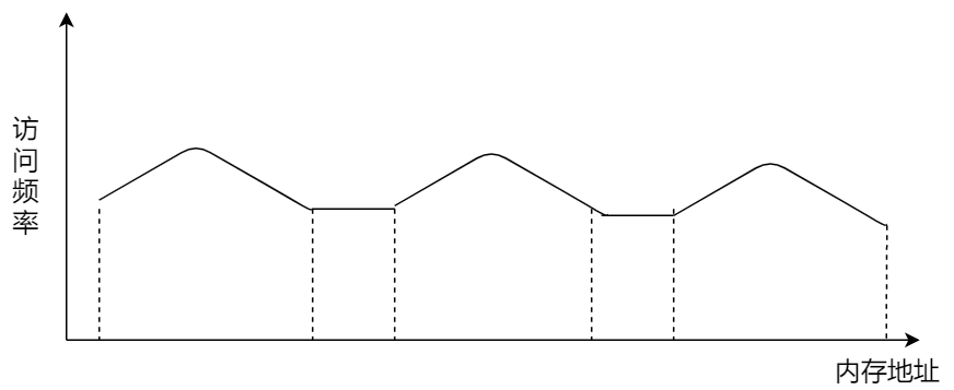
Programs exhibit locality, meaning that within a certain period, the program’s execution is limited to a specific portion of the program. Correspondingly, the memory space accessed during execution is also confined to a certain memory region.

We can leverage this characteristic by storing the most frequently accessed page table entries in faster-access hardware. So, computer scientists introduced a Cache within the CPU chip designed specifically for storing the program’s most frequently accessed page table entries. This cache is called the TLB (Translation Lookaside Buffer), commonly referred to as a page table cache, translation buffer, or fast table, among other names.

Within the CPU chip, there is an encapsulated component called the Memory Management Unit (MMU), which is responsible for performing address translation and interacting with the TLB (Translation Lookaside Buffer).

With the TLB in place, when the CPU is addressing memory, it first checks the TLB. If it doesn’t find the needed information there, it then proceeds to check the regular page tables.

In practice, the TLB has a high hit rate because programs frequently access only a few pages.

4 Segmented Paging Memory Management

摘录自20 张图揭开「内存管理」的迷雾，瞬间豁然开朗

Memory segmentation and memory paging are not mutually exclusive; they can be combined and used together in the same system. When combined, this is typically referred to as segmented paging memory management.

The implementation of segmented paging memory management is as follows:

1. Firstly, divide the program into multiple segments with logical significance, as mentioned earlier in the segmentation mechanism.
2. Then, further divide each segment into multiple pages, which means dividing the contiguous space obtained through segmentation into fixed-sized pages.

As a result, the address structure consists of segment number, page number within the segment, and page offset.

The data structures used for segmented paging address translation include a segment table for each program, and for each segment, a page table is established. The addresses in the segment table point to the starting address of the page table, while the addresses in the page table represent the physical page number of a particular page, as shown in the diagram:

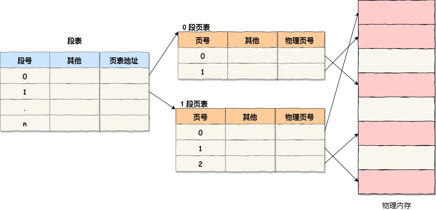
In paged memory addressing, obtaining a physical address requires three memory accesses:

• The first access is to the segment table to obtain the starting address of the page table.
• The second access is to the page table to obtain the physical page number.
• The third access combines the physical page number with the page offset to obtain the physical address.

Segmented paging address translation can be implemented using a combination of software and hardware methods. While this increases hardware costs and system overhead, it improves memory utilization.

5 Linux Memory Management

摘录自20 张图揭开「内存管理」的迷雾，瞬间豁然开朗

So, what method does the Linux operating system use to manage memory?

Before answering this question, let’s take a look at the development history of Intel processors.

Early Intel processors, starting from the 80286, used segmented memory management. However, it was soon realized that having only segmented memory management without paging would not be sufficient, and this would make the x86 series lose its competitiveness in the market. Therefore, paging memory management was implemented shortly after in the 80386. In other words, the 80386 not only continued and improved upon the segmented memory management introduced by the 80286 but also implemented paging memory management.

However, when designing the paging memory management of the 80386, it did not bypass segmented memory management. Instead, it was built on top of segmented memory management. This means that the role of paging memory management is to add another layer of address mapping to the addresses mapped by segmented memory management.

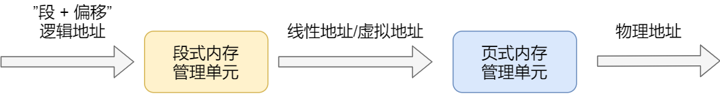
Since the addresses mapped by segmented memory management at this point are no longer “physical addresses,” Intel referred to them as “linear addresses” (also known as virtual addresses). Therefore, segmented memory management first maps logical addresses to linear addresses, and then paging memory management maps linear addresses to physical addresses.

Here, let’s explain logical addresses and linear addresses:

• The addresses used by programs, usually those not mapped by segmented memory management, are called logical addresses.
• Addresses mapped through segmented memory management are called linear addresses, also known as virtual addresses.

Logical addresses are the addresses before the transformation by segmented memory management, while linear addresses are the addresses before the transformation by paging memory management.

After understanding the development history of Intel processors, let’s discuss how Linux manages memory.

Linux primarily uses paging memory management, but it unavoidably involves the segment mechanism as well.

This is mainly due to the historical development of Intel processors mentioned above because Intel X86 CPUs first perform segmented mapping on the addresses used in programs before they can be subjected to paging mapping. Since the CPU’s hardware structure is this way, the Linux kernel has no choice but to adhere to Intel’s choice.

However, in practice, the Linux kernel ensures that the segmented mapping process effectively has no impact. In other words, when there are policies from above, there are also countermeasures from below. If you can’t confront it, you evade it.

In the Linux system, each segment starts from address 0 in the entire 4GB virtual space (in a 32-bit environment). This means that all segments have the same starting address. Consequently, the address space faced by code in the Linux system, including the code of the operating system itself and application code, is all linear address space (virtual address). This approach essentially masks the concept of logical addresses in the processor, and segments are only used for access control and memory protection.

Now, let’s take a look at how the virtual address space in Linux is distributed.

In the Linux operating system, the virtual address space is internally divided into two parts: kernel space and user space, and the range of the address space varies for different bit systems, such as the most common 32-bit and 64-bit systems, as shown below:

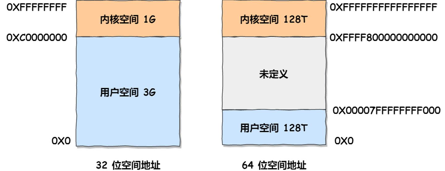
From this information, we can observe the following:

• In a 32-bit system, the kernel space occupies 1GB at the highest end, leaving 3GB for the user space.
• In a 64-bit system, both the kernel space and user space are 128TB, occupying the highest and lowest portions of the entire memory space, with the middle portion left undefined.

Now, let’s talk about the differences between kernel space and user space:

• When a process is in user mode, it can only access memory within the user space.
• Only when a process enters kernel mode can it access memory within the kernel space.

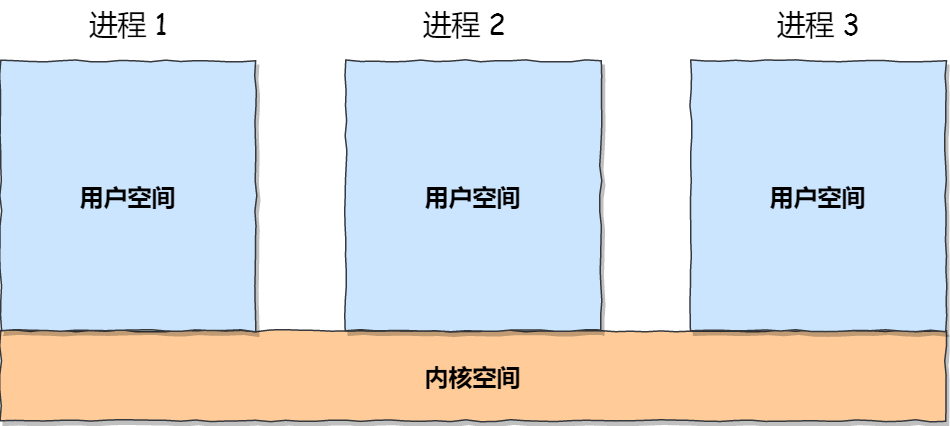
Although each process has its own independent virtual memory, the kernel addresses within each virtual memory are actually associated with the same physical memory. This allows processes to conveniently access kernel space memory when they switch to kernel mode.

Next, let’s further explore the partitioning of the virtual space. The division between user space and kernel space is different, so we won’t delve into the distribution of kernel space.

Let’s take a look at how user space is divided. I’ve created a diagram to illustrate their relationship, using a 32-bit system as an example:

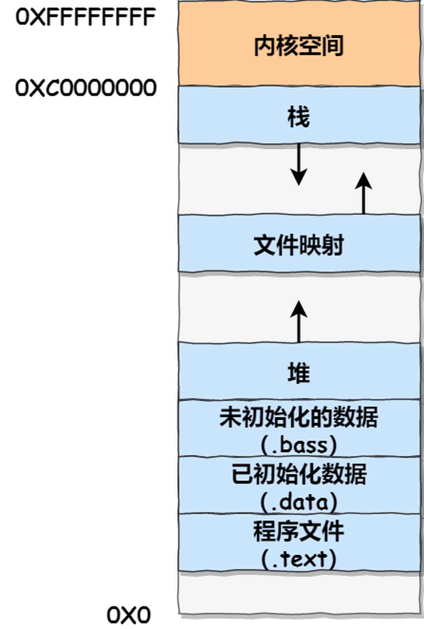
From this diagram, you can see that user space memory is divided into 7 different memory segments from low to high:

• Program File Segment, including binary executable code.
• Initialized Data Segment, including static constants.
• Uninitialized Data Segment, including uninitialized static variables.
• Heap Segment, including dynamically allocated memory, which grows upwards from a low address.
• File Mapping Segment, including dynamic libraries, shared memory, etc., which also grows upwards from a low address (depending on hardware and kernel version).
• Stack Segment, including local variables and the context of function calls. The stack size is typically fixed, often around 8MB, although the system provides parameters for customizing the size.
• Among these 7 memory segments, the memory in the Heap and File Mapping segments is dynamically allocated. For instance, you can use the malloc() function from the C standard library or mmap() to dynamically allocate memory in the Heap and File Mapping segments, respectively.

5.1 How logical addresses are converted to physical addresses

摘录自线性地址转换为物理地址是硬件实现还是软件实现？具体过程如何？

Memory addresses that appear in machine language instructions are logical addresses. They need to be converted into linear addresses and then passed through the Memory Management Unit (MMU), which is a component within the CPU responsible for memory management, in order to access physical memory.

Let’s take a look at the simplest “Hello World” program. When we compile it with GCC and then disassemble it, we will see the following instructions:

mov 0x80495b0, %eax

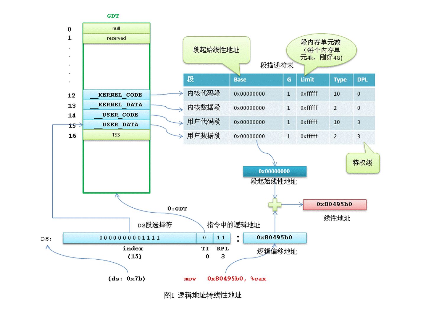
The memory address 0x80495b0 mentioned here is a logical address. To form a linear address, it must be combined with the implicit base address of the DS data segment. In other words, 0x80495b0 is an offset within the DS data segment of the current task.

In the x86 protected mode, segment information (segment base linear address, length, permissions, etc.), known as segment descriptors, occupies 8 bytes. Segment information cannot be directly stored in segment registers (segment registers are only 2 bytes). Intel’s design is to store segment descriptors in a centralized manner in the Global Descriptor Table (GDT) or Local Descriptor Table (LDT), while the segment registers hold the index of the segment descriptor within the GDT or LDT.

In Linux, logical addresses are equal to linear addresses. Why is this the case? Because in Linux, all segments (user code segment, user data segment, kernel code segment, kernel data segment) have linear addresses starting from 0x00000000 with a length of 4GB. So, linear address = logical address + 0x00000000, meaning that logical addresses are effectively equal to linear addresses.

As evident from the above, Linux operates on the x86 segment mechanism but cleverly bypasses it. Linux primarily implements memory management through paging.

As mentioned earlier, in Linux, logical addresses are equivalent to linear addresses. To map linear addresses to physical addresses, the paging mechanism is used. More precisely, it’s the CPU that provides the paging mechanism, and Linux uses it to implement memory management.

In protected mode, the highest bit of the control register CR0, known as the PG bit, controls whether the paging mechanism is active. If PG=1, the paging mechanism is active, and linear addresses must be translated into physical addresses through page table lookups. If PG=0, the paging mechanism is inactive, and linear addresses are used directly as physical addresses.

The fundamental principle of paging is to divide memory into fixed-size units called pages, with each page containing 4KB of address space (ignoring extended paging for simplicity). Thus, each page starts at an address that is aligned to a 4KB boundary. To translate linear addresses into physical addresses, a page table (or page directory in the case of two-level paging) is provided for each task. Note that to achieve a flat virtual memory for each task, each task has its own page directory and page table.

To save memory space, x86 divides a 32-bit linear address into three parts:

• The highest 10 bits (Directory) represent the page directory offset.
• The middle 10 bits (Table) represent the page table offset.
• The lowest 12 bits (Offset) represent the byte offset within the physical page.

The page directory table has a size of 4KB (exactly one page), with 1024 entries, each of 4 bytes (32 bits). Each entry stores the physical address of the page table. If the page table for a specific entry has not been allocated, the physical address is set to 0.

The page table also has a size of 4KB, containing 1024 entries, each of 4 bytes, with each entry containing the physical memory start address for the final physical page.

For each active task, a page directory table must be allocated, and its physical address is stored in the CR3 register. Page tables can be allocated in advance or on-demand as needed.

Now, let’s analyze the process of translating a linear address into a physical address using the example address mov 0x80495b0, %eax.

As mentioned earlier, Linux treats logical addresses as linear addresses, so the address we need to convert is 0x80495b0. The CPU automatically performs this conversion, and Linux’s role is to prepare the necessary page directory and page tables (assuming they have been prepared; the process of allocating physical memory for page directory and page tables is complex and will be analyzed later).

The kernel first places the physical address of the current task’s page directory table into the CR3 register.

The linear address 0x80495b0 in binary is 0000 1000 0000 0100 1001 0101 1011 0000. The highest 10 bits, 0000 1000 00, represent decimal 32. The CPU looks up the 32nd entry in the page directory table, which contains the physical address of the page table. The middle 10 bits, 00 0100 1001, represent decimal 73. The 73rd entry in the page table contains the physical start address of the final physical page. By adding the physical page base address to the lowest 12 bits of the linear address, the CPU finds the physical memory unit corresponding to the linear address.

In Linux, user process linear addresses can address a range from 0 to 3GB. Does this mean we need to pre-allocate page tables for this entire 3GB virtual memory range? In most cases, physical memory is much smaller than 3GB, and multiple processes are running concurrently, making it impractical to pre-allocate 3GB of page tables for each process. Linux addresses this issue using a CPU mechanism. After a process is created, we can set the values in the page directory table entries to 0. When the CPU looks up a page table and finds a table entry with a content of 0, it triggers a page fault exception. The process is temporarily suspended, and the Linux kernel, through a series of complex algorithms, allocates a physical page and fills the entry with the physical page’s address. The process then resumes execution. During this process, the process is unaware and still believes it is accessing physical memory as usual.

6 Summary

1. To address the issue of physical memory addresses causing conflicts between programs and leading to crashes, “Memory Segmentation” or “Segmented Memory Management” was introduced.
2. To overcome the problems of “external fragmentation” and “inefficient memory swapping” associated with memory segmentation, “Memory Paging” or “Paged Memory Management” was introduced.
3. To tackle the issue of “page table space consumption” inherent in memory paging, “Multi-Level Page Tables” were introduced.
4. To achieve “logical program partitioning” while maintaining the advantages of memory paging, “Segmented Paging Memory Management” was introduced.
5. Since segmentation and paging are mechanisms introduced by the CPU, Linux implemented a form of “pseudo-segmented paging memory management,” which is essentially “Paged Memory Management.” In this implementation, all programs and all segments have a base address of 0.

7 Knowledge Fragments

7.1 Related Command Line

1. free
2. vmstat
3. cat /proc/meminfo
4. top
5. slabtop

7.2 buff/cache

7.2.1 What is buffer/cache？

In simple terms, a buffer is used to address the issue of inconsistent read and write speeds. For example, when writing data from memory to a disk, it often needs to be buffered. Cache, on the other hand, is used to address hotspot issues. For instance, when frequently accessing certain hot data, it can be stored in storage media with higher read performance.

Buffer and cache are two widely used terms in computer technology, and they can have different meanings in different contexts. In the context of Linux memory management, “buffer” refers to the buffer cache in Linux memory, while “cache” refers to the page cache in Linux memory. They can be translated into Chinese as “缓冲区缓存” and “页面缓存,” respectively. In the past, “buffer” was used as a write cache for I/O devices, while “cache” was used as a read cache for I/O devices, primarily referring to block device files and regular files in the file system. However, their meanings have evolved over time. In the current kernel, the page cache is a cache specifically for memory pages. In simple terms, any memory managed in pages can use the page cache to manage its caching. Of course, not all memory is managed in pages; some are managed in blocks. This type of memory, if it requires caching, is managed within the buffer cache. (From this perspective, wouldn’t it be better to rename the buffer cache to “block cache”?) However, not all blocks have fixed sizes; the size of blocks on a system depends mainly on the block devices used, while page sizes on x86, whether 32-bit or 64-bit, are always 4k.

7.2.2 What is page cache？

The page cache is primarily used as a cache for file data on the file system, especially when processes perform read/write operations on files. If you think about it carefully, the system call that allows files to be mapped into memory, mmap, also naturally uses the page cache, doesn’t it? In the current system implementation, the page cache is also used as a cache device for other file types. Therefore, in practice, the page cache also handles most of the caching work for block device files.

7.2.3 What is buffer cache?

The buffer cache is primarily designed for use in systems that read and write blocks when interacting with block devices. This means that certain operations involving blocks use the buffer cache for data caching, such as when formatting a file system. In general, these two caching systems work together. For example, when we perform a write operation on a file, the content of the page cache is modified, and the buffer cache can be used to mark pages as belonging to different buffers and record which buffer has been modified. This way, when the kernel performs writeback of dirty data in subsequent operations, it doesn’t have to write back the entire page; it only needs to write back the modified portions.

7.2.4 How to Reclaim

The Linux kernel triggers memory reclamation when memory is about to run out, in order to free up memory for processes that urgently need it. In most cases, the primary source of memory release in this operation comes from releasing buffer/cache, especially the cache space that is used more frequently. Since cache is primarily used for caching and is only intended to speed up file read and write operations when there is enough memory, it is indeed necessary to clear and release the cache when there is significant memory pressure. Therefore, under normal circumstances, we consider that buffer/cache space can be released, and this understanding is correct.

However, this cache clearing process is not without its costs. Understanding what cache is used for makes it clear that clearing the cache must ensure that the data in the cache is consistent with the data in the corresponding files before the cache can be released. Therefore, along with cache clearance, there is usually a spike in system I/O. This is because the kernel needs to compare the data in the cache with the data in the corresponding disk files to ensure consistency. If they are not consistent, the data needs to be written back before reclamation can occur.

How to Clean

1. sync; echo 1 > /proc/sys/vm/drop_caches：Only clean PageCache
2. sync; echo 2 > /proc/sys/vm/drop_caches：Clean dentries and inodes
3. sync; echo 3 > /proc/sys/vm/drop_caches：Clean PageCache, dentries and inodes

7.3 brk and mmap

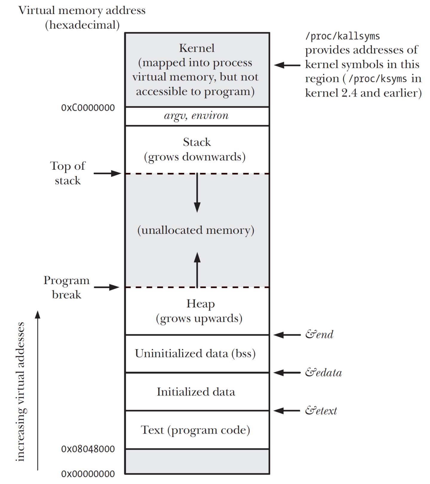
The term “program break” refers to a concept related to memory management in Unix-like operating systems. Specifically, it represents the boundary between the data segment and the heap in a process’s address space. The data segment contains the initialized and uninitialized data of a program, while the heap is used for dynamic memory allocation during program execution.

mmap and brk are both system calls in Unix-like operating systems that are used for memory allocation and management, but they serve different purposes and have some key differences:

• mmap (Memory Mapping):
  • man brk/sbrk
  • Purpose: mmap is primarily used for memory mapping, which allows you to map a file, device, or anonymous memory region into the process’s address space. It can be used for both memory allocation and memory-mapped file operations.
  • Flexibility: mmap is more flexible than brk because it can allocate memory in various ways, including mapping files, devices, and anonymous memory. It allows you to specify the desired size(but the smallest size is a single page, typically 4KB), protection, and mapping flags.
  • Use Cases: mmap is commonly used for dynamic memory allocation in modern Unix-like systems, as well as for memory-mapped I/O, shared memory, and memory-mapped files.
• brk and sbrk (Program Break):
  • man mmap/munmap
  • Purpose: brk and sbrk are used for managing the program’s data segment, specifically the end of the data segment (program break). They control the size of the heap, which is used for dynamic memory allocation in older Unix programs.
  • Simplicity: brk and sbrk are simpler to use than mmap but have limitations. They allow you to adjust the program’s heap size by moving the program break, effectively allocating or releasing memory. However, they lack the flexibility of mmap in terms of specifying various memory allocation options.
  • Legacy: brk and sbrk are considered legacy and are less commonly used in modern programming because they lack the features and robustness of mmap. Most modern Unix-like systems use mmap or other memory allocation mechanisms for dynamic memory allocation.

In summary, mmap is a more versatile and flexible system call that can be used for various memory allocation and mapping purposes, including dynamic memory allocation. brk and sbrk are older and simpler system calls that control the size of the heap but are less commonly used in modern programming due to their limitations and the availability of more advanced memory management techniques.

And additionally, brk and sbrk allocate virtual memory space within a process’s address space, and the allocation of physical memory pages occurs as data is actually read from or written to the allocated virtual memory.

7.4 Standard File I/O and mmap

Here’s a comparison between “Standard File I/O” and mmap:

1. Access Mechanism:
   • Standard File I/O: Operations involve explicit system calls to read from or write to a file, such as read() and write(). Data is transferred between the kernel space and the user space.
   • mmap: A region of a file is mapped to a region of the process’s memory. After this mapping, reading from or writing to this memory region allows you to directly read from or write to the file. The file access is essentially treated as memory access.
2. Efficiency:
   • Standard File I/O: Each operation, like reading or writing, requires a system call, which introduces some overhead. Additionally, there might be double buffering: one buffer in the application and another in the kernel.
   • mmap: Once a file is memory-mapped, accessing it can be as efficient as accessing regular memory, especially beneficial for random access patterns. No additional system calls are needed after mapping until the memory is unmapped.
3. Use Cases:
   • Standard File I/O: Generally suitable for sequential file operations or when there’s a need for granular control over I/O.
   • mmap: Particularly beneficial for random access patterns, as in some databases or large datasets. It’s also commonly used for inter-process communication (IPC) via shared memory.
4. Memory Management:
   • Standard File I/O: Data is read into buffers managed by the application or the standard library.
   • mmap: Uses the operating system’s page cache directly, potentially avoiding the double-buffering scenario. The OS manages the memory, and can “page out” sections if needed, making it more dynamic.
5. File Size Changes:
   • Standard File I/O: Changing the file size or position isn’t problematic, as you usually check or adjust your position with calls like lseek().
   • mmap: Changing the mapped file’s size can lead to segmentation faults or undefined behavior if not handled correctly.
6. Consistency & Coherency:
   • Standard File I/O: To ensure multiple processes can safely read/write, careful synchronization is often required.
   • mmap: Provides a coherent view of a file. If one process changes a memory-mapped file, another process using the same mapping will see the changes almost immediately.
7. Flexibility:
   • Standard File I/O: Offers a broader range of operations, like different ways to seek within a file, read certain lengths of bytes, or handle errors.
   • mmap: More limited but offers direct memory access benefits.

In conclusion, the choice between Standard File I/O and mmap depends on the specific needs and access patterns of the application. Each has its strengths and ideal scenarios. For simple file reading/writing tasks, Standard File I/O is often sufficient. For performance-critical applications with specific patterns, mmap can offer advantages.

7.5 TLB shootdown

A TLB (Translation Lookaside Buffer) shootdown is a mechanism used in multiprocessor computer systems to ensure the consistency of virtual-to-physical address mappings in the TLB cache of each processor.

Let’s break this down a bit:

1. What is a TLB?: The Translation Lookaside Buffer (TLB) is a hardware cache that stores recent virtual-to-physical address translations. When a processor needs to access data, it does so using a virtual address. The TLB checks to see if it has a recent translation for that virtual address to a physical address in memory. If it does (a TLB hit), the processor can access the data faster. If it doesn’t (a TLB miss), the system needs to fetch the translation from the page tables, which is slower.
2. Why is consistency needed in a multiprocessor system?: In multiprocessor systems, each processor typically has its own TLB. If one processor changes a virtual-to-physical mapping (e.g., because of memory management operations like paging or memory unmapping), other processors’ TLBs might still have the old, now-stale mapping.
3. What is a TLB shootdown?: A TLB shootdown is a procedure to ensure that when a virtual-to-physical mapping is changed or invalidated on one processor, other processors are informed and can update or invalidate their own TLBs as needed. This process ensures that all processors have a consistent view of memory.
4. How does it work?: When a processor modifies a page table entry that might be cached in other processors’ TLBs, it sends an inter-processor interrupt (IPI) to the other processors. This IPI acts as a signal to those processors to check and, if necessary, invalidate their local TLB entries for the given virtual address. The term “shootdown” arises because it’s as if the initiating processor is telling the other processors to “shoot down” any potentially stale TLB entries they have.
5. Performance Implications: TLB shootdowns can have a performance impact because they involve synchronization between processors. Each IPI can cause a processor to be interrupted from its current task, handle the invalidation request, and then resume its task. If TLB shootdowns are frequent, they can degrade system performance. Thus, optimizing and reducing the frequency of TLB shootdowns is an area of focus in operating system and hardware design.

In summary, a TLB shootdown is a synchronization mechanism used in multiprocessor systems to ensure that all processors have a consistent and up-to-date view of virtual-to-physical address translations.

7.6 Slab Allocation

The term “slab allocation” refers to a memory management mechanism implemented in certain operating systems, notably the Linux kernel. Its primary goal is to efficiently manage memory allocations by caching objects of frequently used fixed sizes to avoid the overhead of constantly allocating and deallocating small chunks of memory.

Here’s a breakdown of slab allocation:

1. Problem with Fragmentation: When a system frequently allocates and deallocates small chunks of memory, it can lead to fragmentation. This means that while there might be free memory available, it’s scattered in small chunks throughout the system, making it unusable for larger allocations.
2. The Concept of Caches: To solve the fragmentation issue and to optimize the allocation and deallocation processes, the slab allocator introduces the concept of caches. Each cache is designed to hold objects of a specific size.
3. Slabs: Within each cache, memory is organized into “slabs.” A slab is a contiguous block of memory divided into equally sized parts that fit objects of the cache’s designated size. Slabs can be in one of three states:
   • Empty: All objects are free.
   • Partial: Some objects are allocated, and some are free.
   • Full: All objects are allocated.
4. Allocation & Deallocation: When the system requires an object of a particular size, it looks for a suitable cache and then checks for a free object in one of the partial slabs (or an empty slab if no partial slabs have free objects). When objects are deallocated, they are returned to their slab, making them available for future allocations. This mechanism reduces the overhead of frequently carving out and reclaiming small chunks of memory.
5. Benefits:
   • Reduces fragmentation.
   • Speeds up memory allocation for commonly sized objects.
   • Makes the deallocation process efficient.
6. Usage in Linux: The Linux kernel uses the slab allocator for various purposes, including allocating kernel objects like inode and dentry structures, which have fixed sizes and are frequently allocated and deallocated.

The slab allocation strategy is just one approach to kernel memory management. There are other strategies like the slob (simple list of blocks) and slub (the unqueued slab allocator) allocators in the Linux kernel, each with its advantages and trade-offs.

8 Reference

• 20 张图揭开「内存管理」的迷雾，瞬间豁然开朗
• 线性地址转换为物理地址是硬件实现还是软件实现？具体过程如何？
• How to Clear RAM Memory Cache, Buffer and Swap Space on Linux
• Linux使用free命令buff/cache过高
• linux内存占用问题调查——slab
• How much RAM does the kernel use?
• Linux系统排查1——内存篇
• 深入理解 Linux 内核–jemalloc 引起的 TLB shootdown 及优化